TL;DR

Whilst there is software already out there that can analyse physical activity data files, we have found that taking a raw .csv file and calculating intensity categories can be a great way to understand how counts are converted into minutes of behaviour. It also is also a good opportunity to put into practice some of the things we covered during the data transformation posts.

Introduction

Calculating minutes of behaviour from wearable devices such as accelerometers is something that we do quite a lot within our research. Normally this would be completed within software such as ActiLife, KineSoft or more recently within R using the package GGIR, but essentially they are just a set of functions that replicate a number of calculations on each file. This tutorial is going to walk you through how to calculate intensity of behaviour from a .csv file whilst using some of the aspects we covered during the transform tutorials.

Accelerometry file processing

For this post we are going to assume you have an interest in this area and are somewhat familiar with accelerometer processing. But if not this review is a good place to start:

Accelerometer Data Collection and Processing Criteria to Assess Physical Activity and Other Outcomes: A Systematic Review and Practical Considerations (Migueles et al. 2017)

But converting counts into more physiologically relevant units of minutes of behaviour is one of the primary aims of acceleromtry processing. Software does this automatically depending on the criteria you choose but you can do it manually too. This is exactly something we have taught students in the past to demonstrate the process as it can be difficult to understand when a piece of software does everything for you.

Preparing the file

Depending on which accelerometer you use will dictate what file is exported, but for the purpose of this tutorial, we will be using a .csv file from an ActiGraph device that was worn at the waist for seven days. We aren’t covering how this is exported but in short, we have converted a .gt3x file into a .csv and aggregated it to a 60 second epoch. Download the below file and read it into R for the post.

padata.csv

Accelerometry .csv file

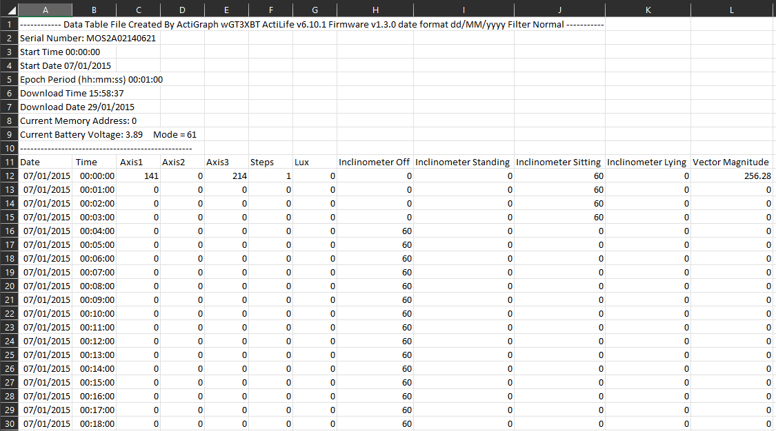
The data is structured to include a header section (rows 1-10) which includes important information about the device that was used, the deployment date and a couple of other bit of information that may be useful. This particular ActiGraph device (wGT3XBT) was deployed for up to 7 full days and has been exported into a 60 second epoch file. Other aspects to be aware of are:

Date: The date of each entry in the list.
Time: The minute epoch for each entry in the list. Each minute will have a its own date and time attached to it.
Axis 1-3: These are the count value that has been recorded in the 3 axes (x, y & Z) for that minutes. For count based accelerometry, these will be the values we will be using to determine the average intensity per minute which will then be summed to provide us with minutes of behaviour per day.
Steps: The step count for the minutes.
Lux: The light sensor entry which may include values if enabled on the device.
Inclinometer: this sensor detects the average posture for the wearer for each minute. This can be used but with other devices specifically set up to measure this (activPAL), the data is not often used.
Vector Magnitude: In earlier device, there was only one axis captured. WIth the development of tri-axial monitors, the vector magnitude represents the square root of the sum of the squares of each axis of data and can also be used for behavioural estimation. When you see behavioural thresholds that use this term, that is what it means.

Now you know what each variable represents, it is time to read the file into RStudio.

gludata <- read.csv("./static/files/padata.csv", header=FALSE)
#The above code is specific to this post
#First, either create a project and move the downloaded file to your project directory or set your working directory where file are located e.g. C:/Users/username/Downloads
#Then use the read.csv code as in the above referenced post
#We have used the header=FALSE option to import the file as it is

Now you have loaded the data we can clean it using the code below.

library(dplyr)
#load the required package
gludata <- gludata %>%
  slice(-c(1:11)) %>%
  select(-c(4:12)) %>%
  dplyr::rename(date = V1, time = V2, axis1 = V3) %>%
  mutate(date = as.POSIXlt(date, format = "%d/%m/%Y")) %>%
  mutate(axis1 = as.numeric(axis1))
#slice removes the header information and filter removes the necessary variables
#dplyr::rename changes the names of the variables back to what they should be after the import
#this is slightly different to previous tutorials as there appeared to be a conflict with the package when running the code multiple times and so the :: specifies that you want to use the function from dplyr
#mutate changes the chr date to a date variable and axis1 to numeric

After running the above code you should now have three variables including Date, Time and Axis 1. We have selected Axis 1 as this is the axis that cut-points have historically been developed from. We also imported the whole file as it was but you could have removed the header before import and by using the header=TRUE code you wouldn’t need to use the rename function. Now the next thing to do is calculate intensity

Calculating intensity

A high level overview of accelerometry is to convert proprietary units called counts into more physically relevant units of minutes of behaviour. To do this, researchers have developed cut-points of thresholds that define when one behaviour moves from one intensity to the other. Now we know that this doesn’t really happen in practice (the same run could be categorised as three different intensities if the data was right) it gives researchers an idea of the behavioural patterns of an individual and any errors will likely be averaged out over the entire file.

One of the most commonly used set of cut-points for adults was developed by Troiano et al. 2008 but in short:

Sedentary = 0 - 99 counts per minute (CPM)
Light = 100 - 2019 CPM
Moderate = 2020 - 2998 CPM
Vigorous = 5999 - infinity CPM

In practice, researchers are most interested in minutes of moderate to vigorous physical activity and so collapse the moderate and vigorous categories to >2020 CPM. Hopefully you will now see that all the cut-points do is tell the software to categorise each minute of data into a particular behaviour based upon its count value. This is a basic version of acceleromtry processing and there are other rules and decisions to make along the way. But in my experience, showing how the minutes are derived from a .csv allows you to start to see how the decisions influence your results. So we won’t get bogged down in the measurement nuance and proceed to calculate minutes of behaivour within the above thresholds.

gludata <- gludata %>%
  mutate(intensity = ifelse(between(axis1, 0, 99), "0-sedentary", 
                     ifelse(between(axis1, 100, 2019), "1-light", 
                     ifelse(between(axis1, 2020, 2998), "2-moderate", "3-vigorous"))))
#This asks R to create a new variable called intensity and then label each row depending on the value within Axis1
#These numbers are the Troiano 2008 cut-point numbers
#We have included numbers before each intensity label for ordering later on

You should now see a new variable called intensity that has placed a number a number between 0 and 3 next to each row. This number corresponds to an intensity with 0 = sedentary and 3 = vigorous.

The next step is to summarise the column by day to see the total amount of behaviour within each of the cut-point categories.

gludata <- gludata %>%
            group_by(date) %>%
            mutate(day = cur_group_id()) %>%
            ungroup()
#For ease, we have created a new day variable which provides a sequential number to each day

library(reshape)
#You need to install this first before running the code
#This is required to reshape the summarise from a long format into a wide format

#group_by groups the table by intensity and day
#summarise n() counts how many rows there are per intensity and day
#cast reformats the data into a table so each row is a new intensity and each column is a new day
results <- gludata %>%
  group_by(intensity,day) %>%
  summarise(n = n()) %>%
  cast(intensity~day) %>%
  ungroup()
print(results)

##     intensity    1    2   3    4    5    6    7
## 1 0-sedentary 1127 1073 989 1170 1182 1097 1109
## 2     1-light  299  309 391  242  254  301  270
## 3  2-moderate   13   24  17    4    3   16   15
## 4  3-vigorous    1   34  43   24    1   26   46

In the above code you will have noticed that we created a new variable called day. This was because it gets a bit tricky to group by dates in R and it is far easier to create a new factor variable. Also, we introduced a new package called ‘reshape’ to restructure the data from the summarise function. If you remove the “cast()” bit from the code the output will show you the results in a long format i.e. each intensity and day in a new row. This package therefore rearranges the data so that each row is an intensity and then each new column is a new day.

For those that are somewhat familiar with accelerometry processing you can see that on average this individuals completes 267 minutes of moderate to vigorous physical activity per week which is much more than the guidelines of 150 minutes per week. You should have also noticed that this person spends on average 18.5 hours sedentary per day… which doesn’t make a lot of sense.

Well the above code that we have used is quite basic and the sedentary category actually includes non-wear time as this individual was asked to remove the device at night when sleeping. Therefore when using accelerometry software, you can use an algorithm to remove any periods of time such as 60 minutes where the device registers no movement. That is a little beyond the scope of this tutorial but we may cover that in future posts.

Conclusion

This post has combined a number of previous tutorials to show you a basic version of accelerometry processing. Actually processing accelerometry data is quite complex and involves a number of difference data processing decisions which we have not covered here. There are a few packages on R that can process your data from accelerometers but these are essential a collection of functions such as the one we have covered here today.

Hopefully you have found this post interesting and that it helps to get your head around how accelerometry data is processed. We hope to cover additional aspects of wearable data processing in the future but if there is something you would like us to cover then please let us know via the contact page.

Complete code

gludata <- read.csv("./static/files/padata.csv", header=FALSE)
#The above code is specific to this post
#First, either create a project and move the downloaded file to your project directory or set your working directory where file are located e.g. C:/Users/username/Downloads
#Then use the read.csv code as in the above referenced post
#We have used the header=FALSE option to import the file as it is

library(dplyr)
#load the required package
gludata <- gludata %>%
  slice(-c(1:11)) %>%
  select(-c(4:12)) %>%
  dplyr::rename(date = V1, time = V2, axis1 = V3) %>%
  mutate(date = as.POSIXlt(date, format = "%d/%m/%Y")) %>%
  mutate(axis1 = as.numeric(axis1))
#slice removes the header information and filter removes the necessary variables
#dplyr::rename changes the names of the variables back to what they should be after the import
#this is slightly different to previous tutorials as there appeared to be a conflict with the package when running the code multiple times and so the :: specifies that you want to use the function from dplyr
#mutate changes the chr date to a date variable and axis1 to numeric

gludata <- gludata %>%
  mutate(intensity = ifelse(between(axis1, 0, 99), "0-sedentary", 
                     ifelse(between(axis1, 100, 2019), "1-light", 
                     ifelse(between(axis1, 2020, 2998), "2-moderate", "3-vigorous"))))
#This asks R to create a new variable called intensity and then label each row depending on the value within Axis1
#These numbers are the Troiano 2008 cut-point numbers
#We have included numbers before each intensity label for ordering later on

gludata <- gludata %>%
            group_by(date) %>%
            mutate(day = cur_group_id()) %>%
            ungroup()
#For ease, we have created a new day variable which provides a sequential number to each day

library(reshape)
#You need to install this first before running the code
#This is required to reshape the summarise from a long format into a wide format

results <- gludata %>%
  group_by(intensity,day) %>%
  summarise(n = n()) %>%
  cast(intensity~day) %>%
  ungroup()
print(results)
#group_by groups the table by intensity and day
#summarise n() counts how many rows there are per intensity and day
#cast reformats the data into a table so each row is a new intensity and each column is a new day

Calculating intensity minutes from a .csv file