Subsetting

For this post we will be using the basic dataset that you will have already seen within post 4.

HStack_data.csv

We will assume that you already know how to read this data into R, but if not we will include the code for you again in the next code segment.

Now there may be a scenario where you may want to reduce your data frame to focus on a subset of participants or you may even want to exclude participants that match a certain criteria. So if we wanted to select only participants based upon age e.g. below 70 from this data set, we would do this using the following code:

data <- read.csv("HStack_data.csv", header = TRUE)
#remember, if you have created a project then move the data file into the project directory

data_sub <- subset(data, Age < 70)
#by running this code you are creating a new dataframe called "data_sub"
#the first part after the ( needs to be the dataframe you are sub setting from and then the condition needs to be specified after the ,
#another example could be to subset by sex e.g. data_sub <- subset(data, Sex == 0) which requires a double = to subset based on an exact value

From using this simple line of code you should now have two data frames, the first with the entire data set and then the second with only 12 participants within it. You should have noticed the comment regarding the use of == to mean equals but if not, this is a useful reminder.

This is one of the most basic ways to sub set your data and can be used to select participants based upon any criteria you choose. However, there are usually multiple criteria that need to be applied and thankfully, all that is required is the “&” symbol. For example:

data_sub <- subset(data, Age < 70 & Sex == 0)
#instead of just selecting by age, a second criteria has also been specified
#in this case there should be 6 participants returned

Other common logical operators include:

• indicates OR
• ! indicates NOT

Also, like everything within R there are other ways to complete the same action which you may come across when using code from other sources:

data_sub <- data[data$Age < 70,]
#using square brackets

However, this comes down to personal preference in the end.

Filtering

The next section of this post will focus on filtering within R but if I am honest, this is just another way of accomplishing what we have just covered (see a theme here??). The only difference with this method is that it requires the use of the dplyr package which we will load within the next code segment. So to achieve the same outcome at the previous section, the following code is required:

library(dplyr)
#load the package

data_sub <- filter(data, Age < 70)
#data_sub is the new data frame
#data is the original source
#the code past the , is the condition

As you can see, you receive the same outcome as you did with the subset code. But where filter comes into its own is when you combine what you have learned from the piping post to reduce the lines of code required. For example:

data_sub <- read.csv("HStack_data.csv", header = TRUE) %>%
  filter(Age <70)
#the file HStack_data.csv should already be in the working directory
#the data frame data_sub is then created using data from the .csv file but has already filtered based upon our set condition

The above has been accomplished using pipes (%>%) and you will notice that because the data source has already been specified within the first line, you do not need to include it within the second line after the pipes. This makes the code a bit easier to understand and removes the need to read in the data THEN create a subset. In addition to the similarities between subset and filter, the logical operators are the same too. By explicitly stating and/or annotating your filter (or subset criteria) within your code makes it easier for other people to see how you have processed the raw data file before your analyses.

Select

We have just covered how to reduce the number of rows (participant) by either using the subset or filter commands within R. But what if you would like to reduce the number of variables within a data frame? Then you can use the select command which comes within dplyr. This is extremely useful if you are presented with a large data set that you would like to read into R, but would only need a few variables from it.

In the case of the data you should still have loaded within your version of R (data), if we would like to only select the height and weight of the participants, this is achieved by the following code:

data_sub <- select(data, ID, Height, Weight)
#the select command words much like filter
#in this case data = the data frame you would like to reduce and the variables you would like to select are listed after the ,

If you are getting the theme of this post, there are other ways to accomplish this and then also achieve it when reading in the data into R such as with the filter command. For example:

data_sub <- select(data, 1,3,4)
#the same action can be accomplished by stating the numeric value of the variable in order that they appear
#the variables can also be selected using the : e.g. 1:4 when within a sequence

data_sub <- select(data, "ID", "Height", "Weight")
#you can also state the name of the variables but this can quite difficult if it is an unknown data set you are using

You will have noticed that the above code always includes the “ID” column and for good reason as it allows for the data to always be traceable. This is especially important if you plan on joining the sub set data frame with additional variables later on but would like to keep the participant ID constant.

Combining data frames

The last thing I will cover within the post is how to join data frames which can especially be useful if you would like to add in additional participants or variables. It goes without saying that you may opt to do this sort of action manually within Excel and then read your data into R, but it is better practice to join data within R using a set key variable. Additionally, whilst you may find manual manipulation easier with a small data set, it becomes unwieldy when there are thousands of participants and/or variables.

Now in R there are different ways to join data frames including:

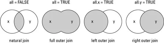
• Inner join (or natural join) - merges data (adds variables) only if rows (IDs) are present in both data frames
• Outer join - merges both variables and rows (IDs)
• Left join - merges data (IDs and variables) from the first data frame with any data (variables) from the second data frame
• Right join - merges data (IDs and variables) from the second data frame with any data (variables) from the first data frame.

This handy graphic from datasciencemadesimple.com nicely explains the above concepts.

However, there are only usually two scenarios when data frames need to be joined in health sciences:

1. when you would like to add variables for all participants to a data frame
2. when you would like to add participants to a data frame.

Now, whilst the first scenario is a join operation, the second actually requires something called a bind function. This is because if you try to conduct an outer join between two data frames that have the same variables names, R will include both variables from data sets 1 and 2 but with suffixes after the variable names. Therefore in this post we will show you how to both join data frames (scenario 1) and bind data frames (scenario 2).

But before we do this, we will create a number of different data sets using the original data frame and then show you how to put them back together again.

library(dplyr)
#load the package

sub1 <- select(data, "ID", "Age", "Grip_strength")
sub2 <- select(data, 1, 3:6)
#creates two data frames which have the same participants (IDs) but different variables

sub3 <- filter(data, Age < 70)
sub4 <- filter(data, Age > 69)
#creates two data frames which have the same variables but different participants (IDs)

The above code has just created 4 different versions of the data frame “data” which all contain either unique participants (sub1 & sub2) or variables (sub3 & sub4).

Now to combine the data frames we just created, you use the following code:

library(dplyr)
#load the package

merged1 <- merge(x = sub1, y = sub2, by = "ID")
#how to conduct an inner join using base R
merged1 <- sub1 %>% inner_join(sub2, by = "ID")
#how to conduct an inner join using dplyr

merged2 <- rbind(sub3, sub4)
#how to merge two datasets together that have the same variables but different participants (IDs)
#you will receive errors if the data frames don’t have the same number of columns or the same column names

After running the above code you now should have the same data reflected within ‘data’, ‘merged 1’ and ‘merged 2’ R objects. A quick check is to look at the number of observations and variables listed next to each object on the Environment tab.

You will have noticed again that you can also use the package dplyr to merge data frames and if you wish to explore the the other types of join, you can use the following snippets of code:

#Inner join base
data <-  merge(x = d1, y = d2, by = "ID", all = FALSE)
#Inner join dplyr
data <- d1 %>% inner_join(d2, by = "ID")

#Outer join base
data = merge(x = d1, y = d2, by = "ID", all = TRUE)
#Outer join dplyr
data <- d1 %>% full_join(d2, by = "ID")

#Left join base
data = merge(x = d1, y = d2, by = "ID", all.x = TRUE)
#Left join dplyr
data <- d1 %>% left_join(d2, by = "ID")

#Right join base
data = merge(x = d1, y = d2, by = "ID", all.y = TRUE)
#Right join dplyr
data <- d1 %>% right_join(d2, by = "ID")