TL;DR

Introduction

The term statistics is often enough to strike fear into most researchers hearts! Hopefully if you are here then this is not the case but if it is do not panic…this post will look to give you a very basic introduction to some of the most common inferential statistics you may want to use. Before we start, lets define the term inferential statistics. Inferential statistics allow us to compare data collected in two groups, often a control group and the treatment/intervention group(s), and from this make generalisations about larger population samples. In this post, we will look at running T-tests and ANOVAs.

T-test

The t-test is a statistical test to analyse the difference in mean between two groups. To perform a t-tests, the data we analyse needs to be parametric in nature. This means that the data needs to follow a normal distribution (if you are unsure what this means, an excellent description is provided here). To assess this we often use a histogram but can also use a statistical test which we will look at below. Lets create our data and then take a look at the distribution. For this post we will create a new dataframe of simulated data. I won’t explain this code in detail as it has no relevance to this post and a small amount of googling should answer any questions you may have.

set.seed(1111) 
#we set the seed so the randomly generated data below is reproducible over time
data <- data.frame(id = c(seq(1, 100)), 
                   intervention = rep(0:1, 50), 
                   mvpa = abs(rnorm(100, mean = 100, sd = 30))) 
#we create a dataframe with an id column of values 1 through 100
#an intervention column with repeating values of 0 and 1
#an mvpa column with normally distributed data with a mean of 100 and a standard deviation of 30
#head is useful to check the dataframe
head(data)

##   id intervention      mvpa
## 1  1            0  97.40260
## 2  2            1 139.67573
## 3  3            0 119.19106
## 4  4            1 135.24360
## 5  5            0 103.48871
## 6  6            1  12.07461

You can see in our dataset that we have 100 participants, 50 of which were assigned to one of two conditions (0 or 1) and we then have an amount of MVPA (moderate to vigorous intensity physical activity) measured. This is a very simplistic dataset, far too simplisitic for any real study however it is enough to be useful for this post. Now we have our data lets take a look at its distribution.

Data distribution

The distribution of our data is important when we look to run certain statistical tests. When we are looking to run a t-test, we need to ensure that our data is normally distributed otherwise we have breached an assumption of our test and our results may not be reliable. If our data is not normally distributed, there are alternative tests that you can run which we will discuss later. For now, lets look at the distribution of our data.

#create a histogram of the mvpa data
hist(data$mvpa)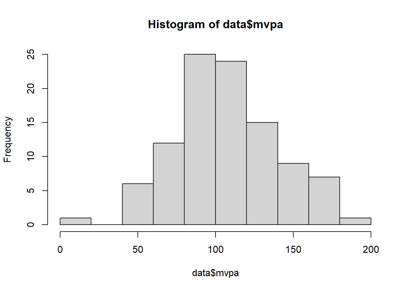

Looking at our histogram, we can see that the data does not follow a traditional normal distribution curve however it does not appear to be skewed in any direction either suggesting it could be normally distributed. To verify our visual inspection, we can also use the Shapiro Wilks test to verify whether our data significantly differs from a normal distribution. To do this in R, we use the shapiro.test function and provide it with our MVPA data.

#run the shapiro-wilks test on the mvpa data
shapiro.test(data$mvpa)

## 
##  Shapiro-Wilk normality test
## 
## data:  data$mvpa
## W = 0.99372, p-value = 0.9276

We can see in the results of this test that the p-value is greater than 0.05 suggesting our data is not significantly different that a normal distribution. Therefore, we are able to progress with our parametric statistical tests assuming our data is normally distributed.

Running a t-test

Now we know are assumptions are met, we can run our t-test. To do this we will use the t.test function from the stats package in R. We provide this function with two arguments. First, we provide it the data from one of our groups, the control group, followed by the data from the intervention group. I use the base R filtering method of square brackets to only include data with a given intervention value. You could however create two separate lists of data each storing the data from one group.

tTestResults <- t.test(data$mvpa[data$intervention == 0], data$mvpa[data$intervention == 1]) 
#run the t.test function by subsetting the mvpa data based on the value of the intervention column
#print the results of the t-test
print(tTestResults)

## 
##  Welch Two Sample t-test
## 
## data:  data$mvpa[data$intervention == 0] and data$mvpa[data$intervention == 1]
## t = 0.25049, df = 95.53, p-value = 0.8027
## alternative hypothesis: true difference in means is not equal to 0
## 95 percent confidence interval:
##  -11.54236  14.87598
## sample estimates:
## mean of x mean of y 
##  108.0786  106.4118

You will notice that I assign the results of the t-test to a variable (tTestResults) and when we print this variable we can see that our p-value is greater than 0.05. Therefore, it appears our intervention did not result in an increase in MVPA.

The reason we assigned the results of the test to an object is we can then access each attribute of the object separately if we need to in the future. For example below, we access the t statistic from the object.

#extract the t value from the tTestResults object
tTestResults$statistic

##         t 
## 0.2504923

This can be particularly useful so you can examine or print out only certain parts of the output. It also allows us to create a table to store the key information from our test if we wanted to.

ANOVA

An ANOVA (ANalysis Of VAriance) is another inferential statistical test which allows us to examine the difference in mean between three groups. Therefore, we will need to make some changes to our previous dataset.

set.seed(123) 
#similar code that was used before the t-test
data <- data.frame(id = c(seq(1, 150)),
                   intervention = rep(0:2, 50), 
                   mvpa = abs(rnorm(150, mean = 100, sd = 30)))
#the same code as before but adds an additional intervention group
#head preview the data
head(data)

##   id intervention      mvpa
## 1  1            0  83.18573
## 2  2            1  93.09468
## 3  3            2 146.76125
## 4  4            0 102.11525
## 5  5            1 103.87863
## 6  6            2 151.45195

We can see in our dataset now that we have three intervention groups represented still with 50 participants in each giving a total of 150 participants. Now we have this simualted dataset, we can look at our distribution.

hist(data$mvpa)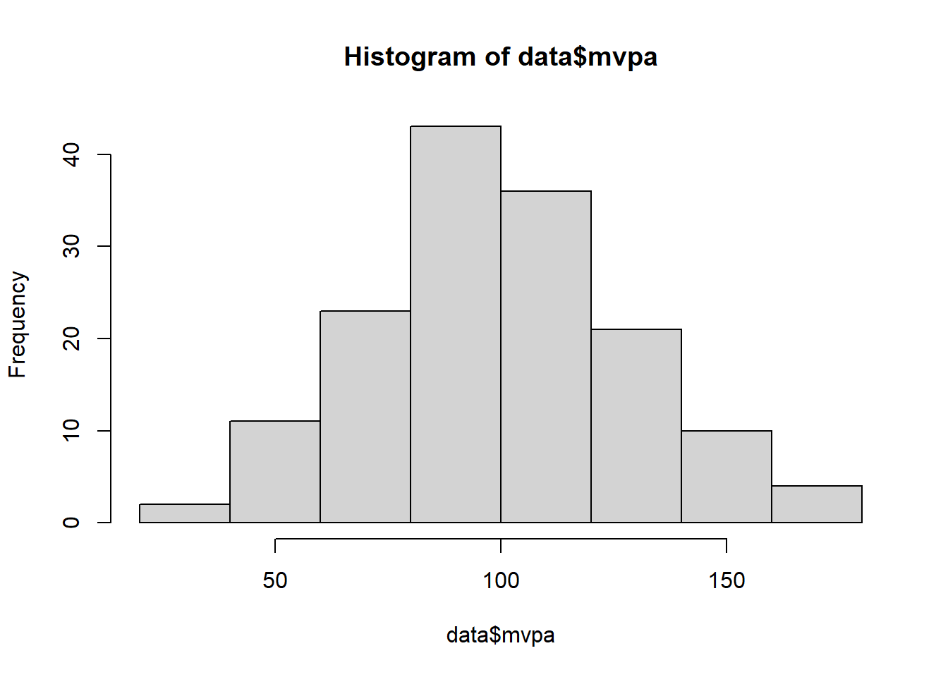

#create a histogram

#conduct a shapiro-wilks test
shapiro.test(data$mvpa)

## 
##  Shapiro-Wilk normality test
## 
## data:  data$mvpa
## W = 0.99239, p-value = 0.6087

We can see from the results of the Shapiro-Wilks test that again we have a p-value greater than 0.05 and therefore we can assume our data is normally distributed and therefore can perform parametric statistical tests. Lets move onto running our ANOVA.

Running an ANOVA

Below is the code required to run an ANOVA in R.

anova <- aov(mvpa[intervention == 0] ~ mvpa[intervention == 1] + mvpa[intervention == 2], data = data) 
#subset the mvpa data based on the value of the intervention column
#summarise the anova object results
summary(anova)

##                         Df Sum Sq Mean Sq F value Pr(>F)
## mvpa[intervention == 1]  1     10     9.8   0.016  0.901
## mvpa[intervention == 2]  1    451   450.7   0.723  0.400
## Residuals               47  29308   623.6

This is slightly more complicated than running the t-test. We use the aov function from the stats package. To this function, we need to supply our data in the format of a formula (the same formula we used when defining linear models). We first provide our control group (in our case participants where intervention is equal to 0), followed by the ~ symbol, and then our two interventions groups separated by a plus sign. We assign the results of our ANOVA to the variable anova. We then run the summary function of the anova object to get the results printed out. By examining the p-values from our test, we can see that neither of our intervention groups had a statistically significant effect on MVPA.

Visualising our tests

Whilst these tests give us a sense of the statistical significance of our data, we may want to provide this information in a more visual way. Boxplots provide a means of doing so.

library(ggplot2)
#set the geom to boxplot
#set the breaks for the x axis
ggplot(data = data, aes(x = intervention, y = mvpa, group = intervention)) +
  geom_boxplot() + 
  scale_x_continuous(breaks = c(0,1,2)) + 
  theme_light()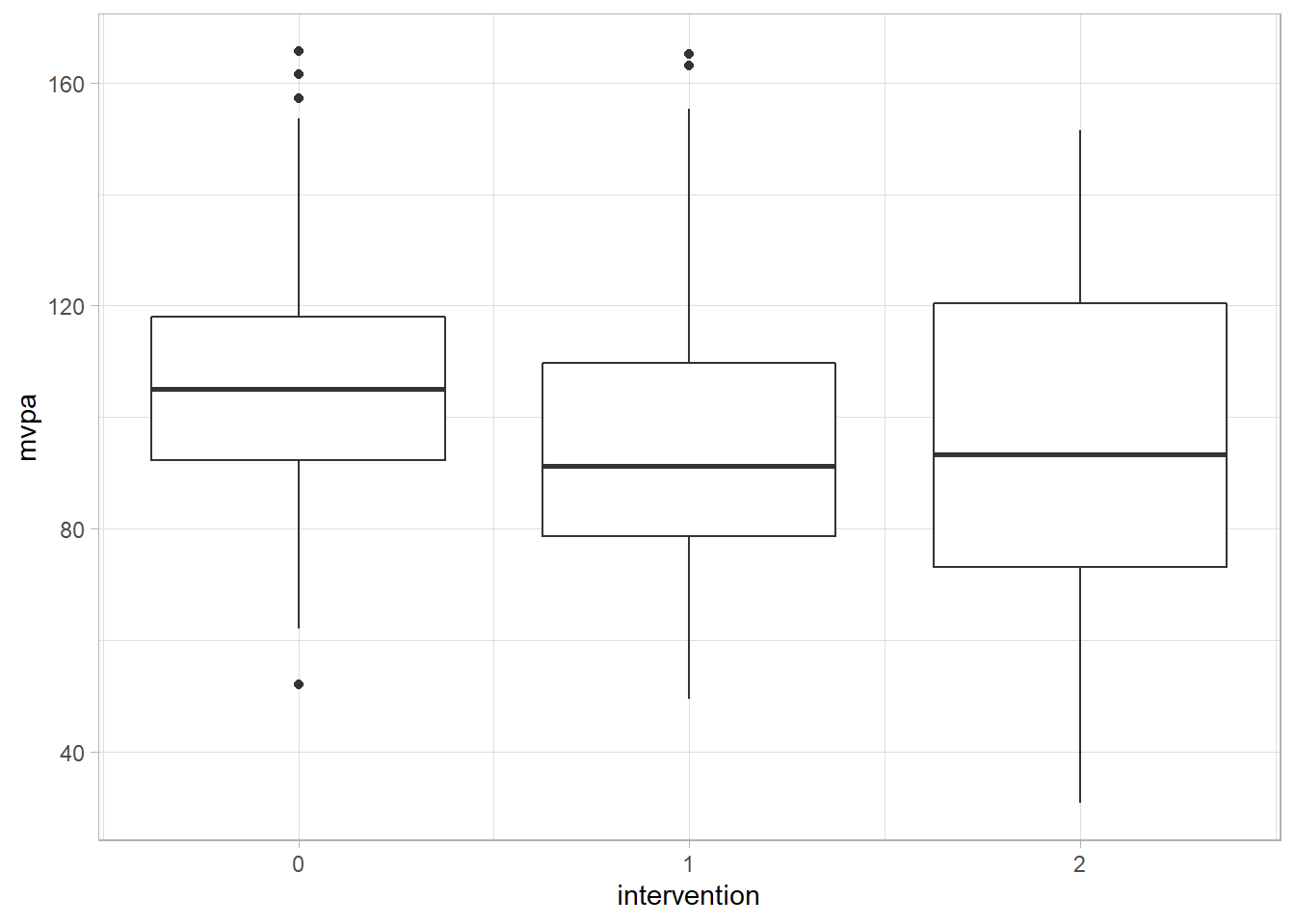

In this rather basic visualisation we can see that the median (the bold line) is higher in group 1 than in the control group (0) and group 2 is higher than both of these groups. However, our ANOVA highlights that these differences are not statistically significant. This highlights that to get a full understanding of our data it is often useful to use the statistical tests and also visually inspect our data.

Non-parametric tests

If your data was to not appear normally distributed, it may not be advisable to use the tests above. Fortunately, there are non-parametric tests that could be substituted for the t-test and ANOVA. For example, a Mann-Whitney U test can be used instead of a t-test to compare two groups whilst a Kruskal-Wallis one way analysis of variance on ranks test can be used in place of an ANOVA. The key difference is that the non-parametric tests utilise the median of the data rather than the mean as the median is less affected by extreme values in the dataset.

A move away from statistical significance?

In recent years, there has been a gradual movement away from solely relying on statistical significance within research. In addition both clinical difference as well as effect sizes are becoming increasing reported. A full discussion of these areas is beyond the scope of this post however this paper offers a more complete explanation of clinically meaningful difference. In terms of effect size, the following paper gives a summary of why using effect size may be better than p-values.

Fortunately, effect sizes are very simple to calculate in R. With the data from our ANOVA lets have a look at the effect size between the control group and intervention group 2.

library(effectsize) 
#library in the effectsize package
#use the cohens_d function from the effectsize package to calculate the effect size 
cohens_d(data$mvpa[data$intervention == 2], data$mvpa[data$intervention == 0])

## Cohen's d |         95% CI
## --------------------------
## -0.40     | [-0.80,  0.00]
## 
## - Estimated using pooled SD.

You can see above that we library in the effectsize package. We then use the cohens_d function from this package to calculate the effect size between our intervention and the control group. We can see from our results that our effect size if 0.38. This would be classed as a small effect size. So although our p-value suggests that there our intervention leads to no statistically significant difference in MVPA, our effect size calculations shows that the intervention actually has a small effect on MVPA.

Conclusions

In the post above we examined how to conduct a t-test and ANOVA within R. We also considered the non-parametric equivalent to these tests and some of the potential alternatives to assessing our data based solely on p-values.

Complete code

set.seed(1111) 
#we set the seed so the randomly generated data below is reproducible over time
data <- data.frame(id = c(seq(1, 100)), 
                   intervention = rep(0:1, 50), 
                   mvpa = abs(rnorm(100, mean = 100, sd = 30))) 
#we create a dataframe with an id column of values 1 through 100
#an intervention column with repeating values of 0 and 1
#an mvpa column with normally distributed data with a mean of 100 and a standard deviation of 30
head(data)
#head is useful to check the dataframe

hist(data$mvpa) 
#create a histogram of the mvpa data

shapiro.test(data$mvpa) 
#run the shapiro-wilks test on the mvpa data

tTestResults <- t.test(data$mvpa[data$intervention == 0], data$mvpa[data$intervention == 1]) 
#run the t.test function by subsetting the mvpa data based on the value of the intervention column
print(tTestResults) 
#print the results of the t-test

tTestResults$statistic 
#extract the t value from the tTestResults object

set.seed(123) 
#similar code that was used before the t-test
data <- data.frame(id = c(seq(1, 150)),
                   intervention = rep(0:2, 50), 
                   mvpa = abs(rnorm(150, mean = 100, sd = 30)))
#the same code as before but adds an additional intervention group
head(data)
#head preview the data

hist(data$mvpa)
#create a histogram

shapiro.test(data$mvpa)
#conduct a shapiro-wilks test

anova <- aov(mvpa[intervention == 0] ~ mvpa[intervention == 1] + mvpa[intervention == 2], data = data) 
#subset the mvpa data based on the value of the intervention column
summary(anova) 
#summarise the anova object results

library(ggplot2)
ggplot(data = data, aes(x = intervention, y = mvpa, group = intervention)) +
  geom_boxplot() + 
  scale_x_continuous(breaks = c(0,1,2)) + 
  theme_light()
#set the geom to boxplot
#set the breaks for the x axis

library(effectsize) 
#library in the effectsize package
cohens_d(data$mvpa[data$intervention == 2], data$mvpa[data$intervention == 0]) 
#use the cohens_d function from the effectsize package to calculate the effect size

Conducting t-tests and ANOVA