TL;DR
Linear models are used frequently in data analysis to examine the relationship between two or more variables. The syntax to define a linear model in R is both easy to write and understand as well as consistent across a wide range of model types. A range of packages provide functions that improve the visual appearance of the model output.
Introduction
Modelling data is a key step in many data analysis pipelines. Data modelling allows us to produce a low level summary of a dataset. It allows us to identify treads and patterns in our data that are not immediately obvious from examining or visualising our dataset. In this post we will take a look at running a basic linear model (also referred to as a linear regression model) and formatting the output.
A basic linear model
For this post, we will use the famous Galton dataset where he examined the relationship between mothers and father height and the height of their children. Let’s start by visually examining our dataset.
galton <- read.csv("~/health_stack/content/post/2021-12-11-conducting-linear-regression-in-r/Galtons Height Data.csv")
#this is the dataset we will be using within this tutorial
#you will need to change the file path to point to the data file on your machine
#we use the base R read.csv function above however there are many other (potentially faster) functions available for larger files
#head views the structure of the dataframe
head(galton)
## Family Father Mother Gender Height Kids
## 1 1 78.5 67.0 M 73.2 4
## 2 1 78.5 67.0 F 69.2 4
## 3 1 78.5 67.0 F 69.0 4
## 4 1 78.5 67.0 F 69.0 4
## 5 2 75.5 66.5 M 73.5 4
## 6 2 75.5 66.5 M 72.5 4If you would like to follow along with this tutorial feel free to download the data below:
You may notice the heights are in inches, I will convert them to centimetres so they are more easily understood by European audiences.
library(dplyr)
library(magrittr)
galton <- galton %>%
  mutate(
    Father = Father * 2.5,
    Mother = Mother * 2.5,
    Height = Height * 2.5
  )
#converting heights to inches
We can see in this dataset we have a family identifier column, the height of the father and mother in inches, the gender of their children, the height of their children and the number of children in each family. Next, let’s visualise our data by creating a graph of mothers height compared to the height of their children.
library(ggplot2)
#visualising the data by creating a graph of mothers height compared to the height of their children
galton %>%
  ggplot(aes(x = Mother, y = Height)) +
  geom_point() +
  geom_smooth(method = "lm", se = FALSE)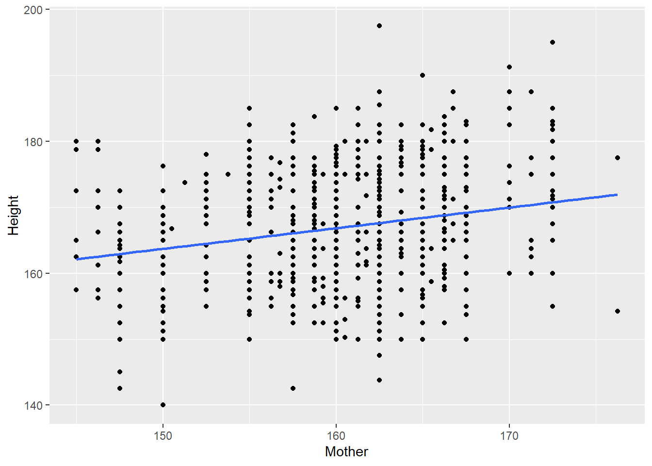
We can see from this graph that there is amn upward trend to our data suggesting that as the height of the mother increases, so does the height of the child. This suggest that it may be worth while to create a linea regression model.
To create a linear model in R, we can use the lm function. The code below creates a model of a child’s height, based on the height of their mother.
child_height <- lm(Mother ~ Height, galton)
#creating a model of a child's height, based on the height of their mother
#lm is a function for linear models from base R
This code has created a linear model object named “child_height”. We can put this into the summary fiunction to summarise our model.
#printing the summary of the linear model
#summary can be applied to many R objects including model objects and dataframes
summary(child_height)
##
## Call:
## lm(formula = Mother ~ Height, data = galton)
##
## Residuals:
## Min 1Q Median 3Q Max
## -16.9118 -3.1133 0.3605 3.8344 17.6817
##
## Coefficients:
## Estimate Std. Error t value Pr(>|t|)
## (Intercept) 138.53972 3.52153 39.341 < 2e-16 ***
## Height 0.12984 0.02107 6.163 1.08e-09 ***
## ---
## Signif. codes: 0 '***' 0.001 '**' 0.01 '*' 0.05 '.' 0.1 ' ' 1
##
## Residual standard error: 5.652 on 896 degrees of freedom
## Multiple R-squared: 0.04066, Adjusted R-squared: 0.03959
## F-statistic: 37.98 on 1 and 896 DF, p-value: 1.079e-09We can see in the above output that we get our beta values (called our Estimate) as well as our standard error, t and P value. We can see that for each centimetre increase in mother height, the child height increase by around 0.13cm. We can also see that this value is highly significant. At the bottom of our summary we can see our adjusted R squared value. This tells us the percentage of the variance in the response variable, in our case childs height, that is explained by the explanatory variable, Mother’s height. In our example, this value is 0.0396 or around 3%. This highlights that Mother’s height explains a very small amount of the variation in children’s height and therefore other variables may need to be added to our model.
The linear model object
I think it is worth taking a few minutes to discuss the linear model object (child_height in our case) which we just created. A model object is fundamentally a list so it can be subsetted using the $ operator. We can extract a lot of information from our model object including the coefficients as below for example.
#a model object is fundamentally a list
#we can use $ to subset model objects in the same way we can dataframes (or named lists)
child_height$coefficients
## (Intercept) Height
## 138.5397222 0.1298447It is well worth taking some time to explore all the outputs you can get from the linear model object as they provide so much more information than what is contained in the model summary. This additional information can be extremely useful when dealing with more complex models or model applications.
Advancing the model
#adding in another term into our model
child_height_2 <- lm(Height ~ Mother + Father, data = galton)
summary(child_height_2)
##
## Call:
## lm(formula = Height ~ Mother + Father, data = galton)
##
## Residuals:
## Min 1Q Median 3Q Max
## -22.8389 -6.7505 -0.4524 6.9210 29.2214
##
## Coefficients:
## Estimate Std. Error t value Pr(>|t|)
## (Intercept) 55.77426 10.76724 5.180 2.74e-07 ***
## Mother 0.28321 0.04914 5.764 1.13e-08 ***
## Father 0.37990 0.04589 8.278 4.52e-16 ***
## ---
## Signif. codes: 0 '***' 0.001 '**' 0.01 '*' 0.05 '.' 0.1 ' ' 1
##
## Residual standard error: 8.465 on 895 degrees of freedom
## Multiple R-squared: 0.1089, Adjusted R-squared: 0.1069
## F-statistic: 54.69 on 2 and 895 DF, p-value: < 2.2e-16We can see in the code above, we use the + operator to add another term into our model. So our model now includes both the height of a childs mother and their father. When examining our beta values, we can see that a 1cm increase in the height of a child’s father appears to be associated with a greater increase in a childs height compared to a 1cm increase in their mothers height (0.38cm vs 0.28cm). We can also see that both our model terms are highly significant. This model also explains significantly more variation in child’s height (10.7%) than our original model.
Beautifying our output
Whilst the above summary outputs are useful for use to explore our models they may not be as useful if we want to communicate our data with others. To help with this, we can use the jtools package. This package generates much more attractive model outputs.
library(jtools)
#we can use the jtools package to generate a much more attractive output
#summ is the jtools version of the summarise function
summ(child_height_2) | Observations | 898 |
| Dependent variable | Height |
| Type | OLS linear regression |
| F(2,895) | 54.69 |
| R² | 0.11 |
| Adj. R² | 0.11 |
| Est. | S.E. | t val. | p | |
|---|---|---|---|---|
| (Intercept) | 55.77 | 10.77 | 5.18 | 0.00 |
| Mother | 0.28 | 0.05 | 5.76 | 0.00 |
| Father | 0.38 | 0.05 | 8.28 | 0.00 |
| Standard errors: OLS |
This is a huge improvement over our previous output which is much more understandable to less technically focused audiences. We can also use the export_summs function from jtools to summarise two models side by side.
#export_summs function from jtools can be used to summarise two models side by side
export_summs(child_height, child_height_2, scale = TRUE)| Model 1 | Model 2 | |
|---|---|---|
| (Intercept) | 160.21 *** | 166.90 *** |
| (0.19) | (0.28) | |
| Height | 1.16 *** | |
| (0.19) | ||
| Mother | 1.63 *** | |
| (0.28) | ||
| Father | 2.35 *** | |
| (0.28) | ||
| N | 898 | 898 |
| R2 | 0.04 | 0.11 |
| All continuous predictors are mean-centered and scaled by 1 standard deviation. *** p < 0.001; ** p < 0.01; * p < 0.05. | ||
Checking model assumptions
There are a number of neat little tricks that can be performed with a model object. One of my favourites is to put the model into the base R plot function.
#checking the assumptions of the model using the plot function
plot(child_height_2)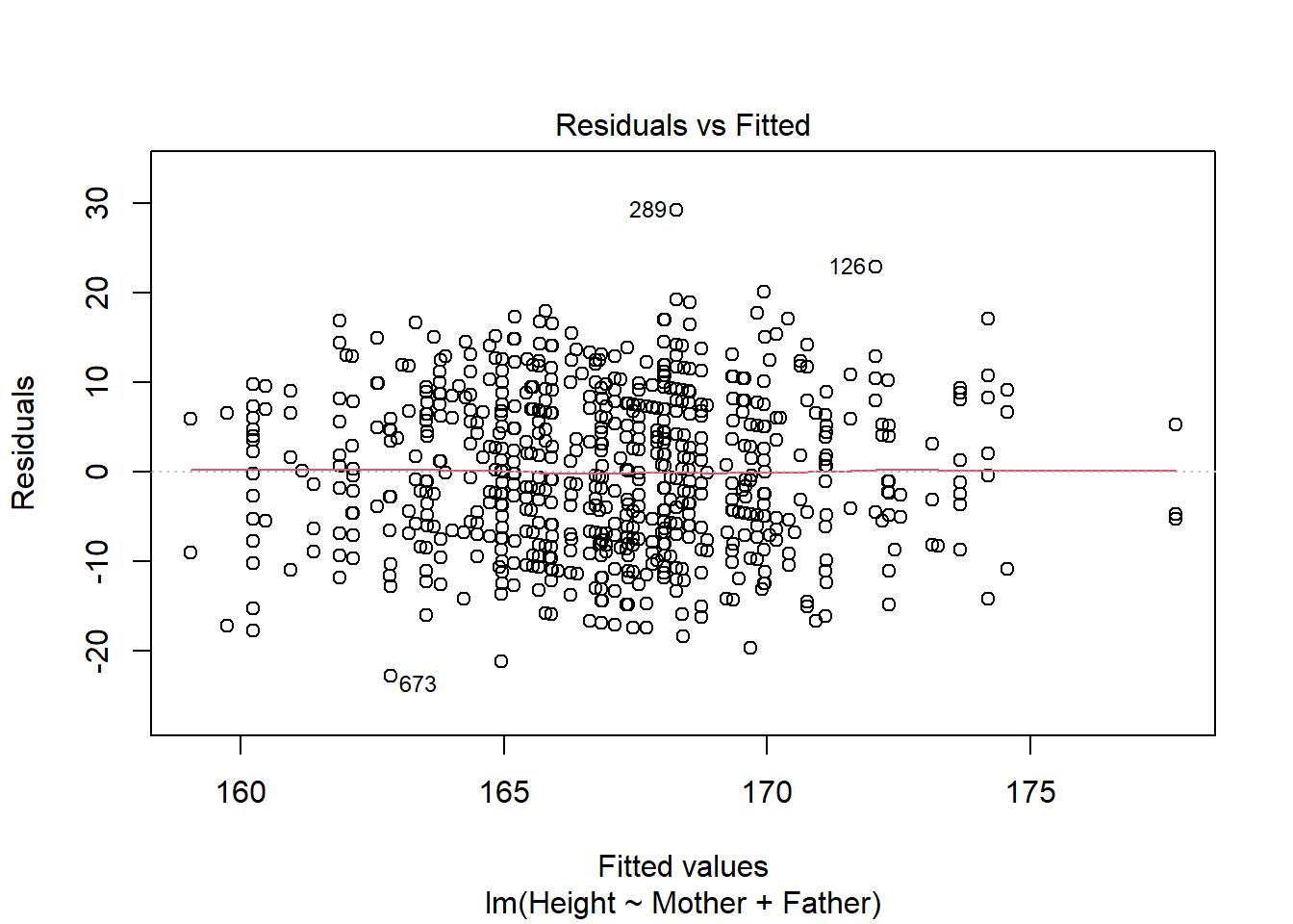
Figure 1: Diagnostic plots for a linear model
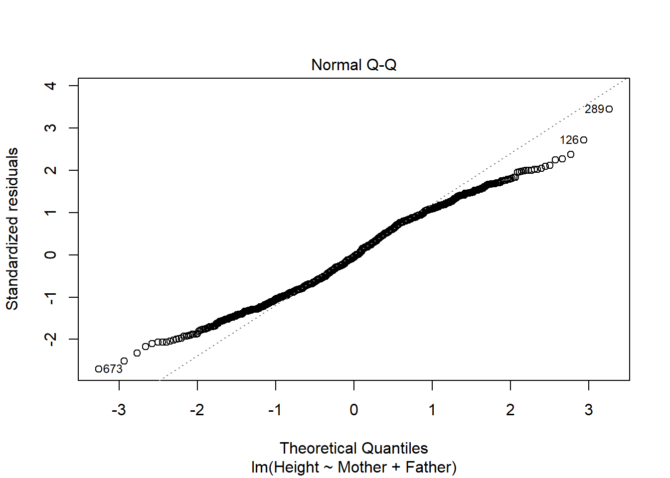
Figure 2: Diagnostic plots for a linear model
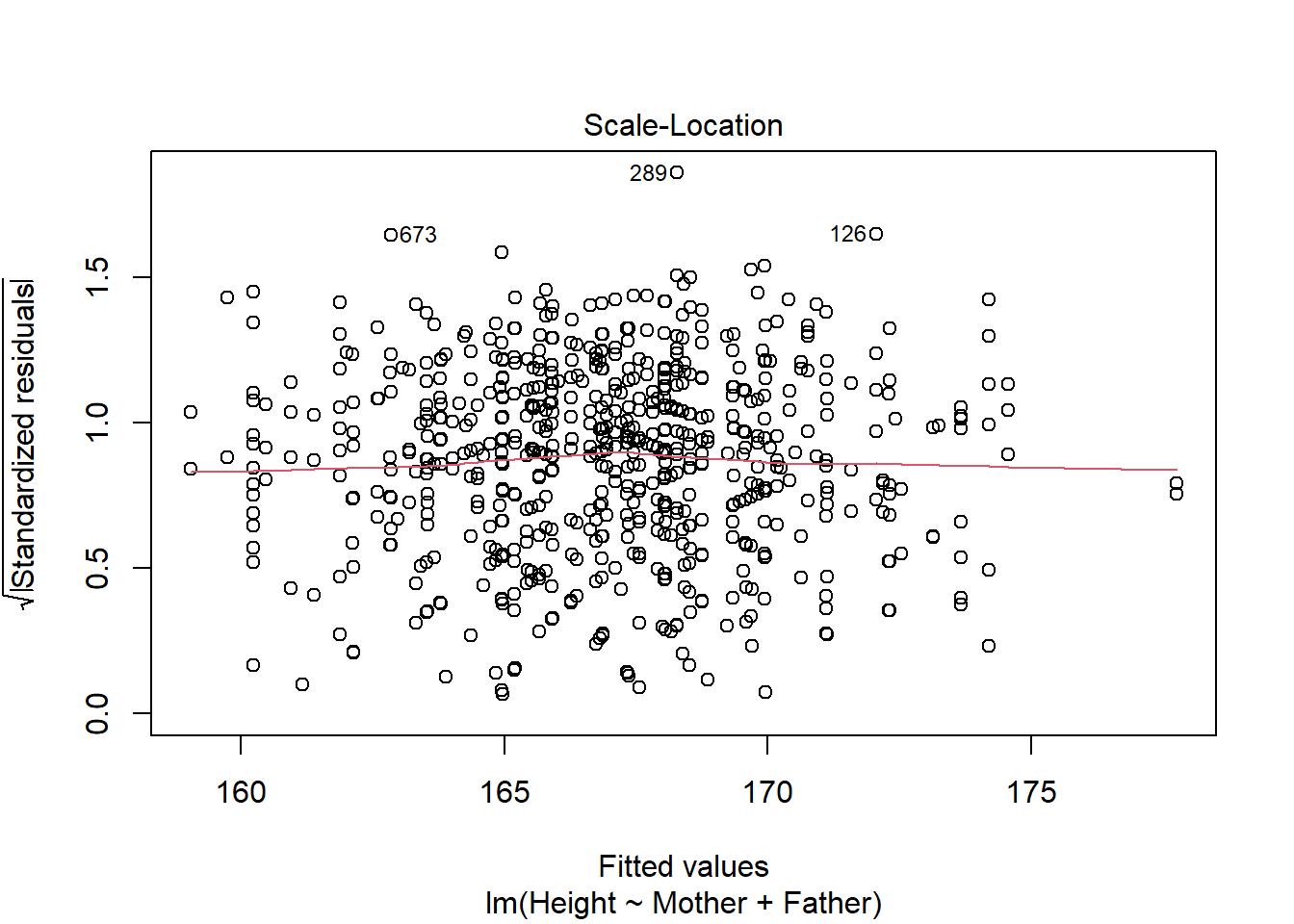
Figure 3: Diagnostic plots for a linear model
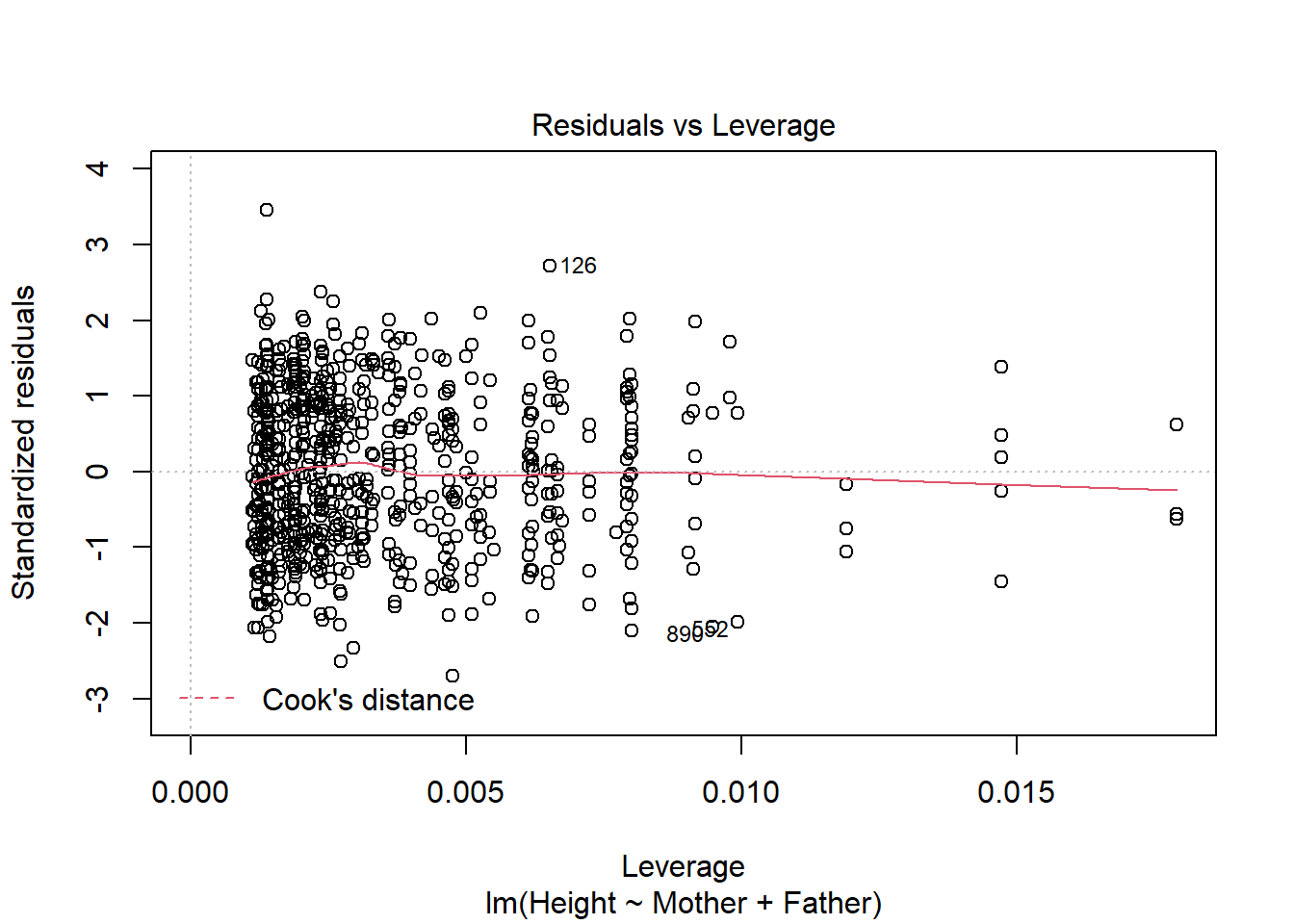
Figure 4: Diagnostic plots for a linear model
This simple line of code creates four graphs by default (however this can be increased to six by setting the which option to c(1,2,3,4,5,6)) which can be used to check the assumptions of a linear model. A complete description of this is outside the scope of this post but can be found here.
Extending our model
The R syntax to define models allows us to do a lot more than just add new model terms. We are also able to add interaction terms using the * operator.
#adding interaction terms into the model
child_height_3 <- lm(Height ~ Mother * Father, data = galton)
summ(child_height_3)| Observations | 898 |
| Dependent variable | Height |
| Type | OLS linear regression |
| F(3,894) | 37.07 |
| R² | 0.11 |
| Adj. R² | 0.11 |
| Est. | S.E. | t val. | p | |
|---|---|---|---|---|
| (Intercept) | 330.87 | 208.02 | 1.59 | 0.11 |
| Mother | -1.43 | 1.29 | -1.10 | 0.27 |
| Father | -1.21 | 1.20 | -1.01 | 0.31 |
| Mother:Father | 0.01 | 0.01 | 1.32 | 0.19 |
| Standard errors: OLS |
Interaction effects in a linear model indicate that the two variables are not independent. This would mean the value of one variable (mothers height) is depends on the value of another variable (fathers height). In our example, this is not the case, however there are really world examples where interaction terms are very useful. We have included this example simply to illustrate their syntax.
Why R makes your life easier
Above we have created linear models using a relatively basic syntax. A major benefit of modelling in R is that the same syntax can be applied to a range of other models. Let’s use the generalised linear model as an example. Such models allow us to predict categorical response variables rather than numeric response variables.
#calculating a generalised linear model using the same syntax
#glm is a base R function for a general linear model
#Before the model is run, the Gender variable needs to be recoded into 0 or 1
#summ from the jtools package creates a visually appealing output
galton <- galton %>%
  mutate(
    Gender = if_else(Gender == "M", 1, 0)
  )
gender <- glm(Gender ~ Height, data = galton, family = "binomial")
summ(gender)| Observations | 898 |
| Dependent variable | Gender |
| Type | Generalized linear model |
| Family | binomial |
| Link | logit |
| χ²(1) | 617.53 |
| Pseudo-R² (Cragg-Uhler) | 0.66 |
| Pseudo-R² (McFadden) | 0.50 |
| AIC | 630.22 |
| BIC | 639.82 |
| Est. | S.E. | z val. | p | |
|---|---|---|---|---|
| (Intercept) | -52.98 | 3.40 | -15.57 | 0.00 |
| Height | 0.32 | 0.02 | 15.57 | 0.00 |
| Standard errors: MLE |
First, we need to recode our Gender variable to be 0 or 1. In our example, we set male (M) to 1 and female (F) to 0. We can then enter this into the glm function and set the model family to binomial meaning our response variable is either one value or the other. We can see in our output that height does have a strong relationship with children’s gender suggesting that males are on average taller than females.
The reason for including this example is to highlight one key point, the R language has a very consistent method to define formulas in a model. This means that once you can create a linear model, you are capable of programming a whole range of other models. This is particularly useful for beginners as you can very rapidly develop a range of modelling techniques.
Conclusion
Linear models are incredibly useful in a range of data analysis pathways. R provides a simple syntax to define models as well as a range of functions to summarise the outputs of the model generated.
Complete code
galton <- read.csv("~/health_stack/content/post/model_linear-regression/Galtons Height Data.csv")
head(galton)
#this is the dataset we will be using within this tutorial
#you will need to change the file path to point to the data file on your machine
#we use the base R read.csv function above however there are many other (potentially faster) functions available for larger files
#head views the structure of the dataframe

library(dplyr)
library(magrittr)
galton <- galton %>%
  mutate(
    Father = Father * 2.5,
    Mother = Mother * 2.5,
    Height = Height * 2.5
  )
#converting heights to inches

library(ggplot2)
galton %>%
  ggplot(aes(x = Mother, y = Height)) +
  geom_point() +
  geom_smooth(method = "lm", se = FALSE)
#visualising the data by creating a graph of mothers height compared to the height of their children

child_height <- lm(Mother ~ Height, galton)
#creating a model of a child's height, based on the height of their mother
#lm is a function for linear models from base R

summary(child_height)
#printing the summary of the linear model
#summary can be applied to many R objects including model objects and dataframes

child_height$coefficients
#a model object is fundamentally a list
#we can use $ to subset model objects in the same way we can dataframes (or named lists)

child_height_2 <- lm(Height ~ Mother + Father, data = galton)
summary(child_height_2)
#adding in another term into our model

library(jtools)
summ(child_height_2)
#we can use the jtools package to generate a much more attractive output
#summ is the jtools version of the summarise function

export_summs(child_height, child_height_2, scale = TRUE)
#export_summs function from jtools can be used to summarise two models side by side

plot(child_height_2)
#checking the assumptions of the model using the plot function

child_height_3 <- lm(Height ~ Mother * Father, data = galton)
summ(child_height_3)
#adding interaction terms into the model

galton <- galton %>%
  mutate(
    Gender = if_else(Gender == "M", 1, 0)
  )
gender <- glm(Gender ~ Height, data = galton, family = "binomial")
summ(gender)
#calculating a generalised linear model using the same syntax
#glm is a base R function for a general linear model
#Before the model is run, the Gender variable needs to be recoded into 0 or 1
#summ from the jtools package creates a visually appealing output