Renaming columns

There are a number of things we may want to check including the variable names within our dataframe.

#get the column names then select the first 5
colnames(mht_data)[1:5] 

## [1] "Are.you.self.employed."                                                           
## [2] "How.many.employees.does.your.company.or.organization.have."                       
## [3] "Is.your.employer.primarily.a.tech.company.organization."                          
## [4] "Is.your.primary.role.within.your.company.related.to.tech.IT."                     
## [5] "Does.your.employer.provide.mental.health.benefits.as.part.of.healthcare.coverage."

Using the colnames functions we can examine the column names within our dataframe. The code above shows us the first five column names and we can see they are rather long and cumbersome. We can rename columns using either base R of dplyr functions.

#base r
names(mht_data)[names(mht_data) == "Are.you.self.employed."] <- "self_employed" 
#get the names of the columns, filter to the column name you want and then assign it a new value

#dplyr
library(dplyr)
mht_data <- mht_data %>%
  rename(employee_n = How.many.employees.does.your.company.or.organization.have.) 
#provide the new variable name, followed by the previous variable name
#recheck the data using the below code
mht_data[1:5, 1:5]

##   self_employed employee_n
## 1             0     26-100
## 2             0       6-25
## 3             0       6-25
## 4             1           
## 5             0       6-25
##   Is.your.employer.primarily.a.tech.company.organization.
## 1                                                       1
## 2                                                       1
## 3                                                       1
## 4                                                      NA
## 5                                                       0
##   Is.your.primary.role.within.your.company.related.to.tech.IT.
## 1                                                           NA
## 2                                                           NA
## 3                                                           NA
## 4                                                           NA
## 5                                                            1
##   Does.your.employer.provide.mental.health.benefits.as.part.of.healthcare.coverage.
## 1                                                   Not eligible for coverage / N/A
## 2                                                                                No
## 3                                                                                No
## 4                                                                                  
## 5                                                                               Yes

Variable type

We may also want to check what type our variables are currently stored in. We can do this using the type_of function.

#check the type of a column
typeof(mht_data$employee_n) 

## [1] "character"

We can see that the number of employees is currently classified as a character vector, however if we examine the content of this variable we will see there are actually six categories and therefore should be considered a factor variable.

mht_data$employee_n <- as.factor(mht_data$employee_n) 
#convert a column to type factor
#examine the levels of a factor
levels(mht_data$employee_n) 

## [1] ""               "1-5"            "100-500"        "26-100"        
## [5] "500-1000"       "6-25"           "More than 1000"

Above we have used the as.factor function to convert the variable from its current type to the type factor. I have then used the levels function to examine how many levels the variable has and the names of these. We now have our factors however you can see they are not in the correct order (6-25 is in the wrong place). We can change this with the code below.

mht_data$employee_n <- factor(mht_data$employee_n, levels = c("1-5", "6-25", "26-100", "100-500", "500-1000", "More than 1000", "")) 
#make the column a factor and set the levels in our chosen order
#examine the levels of a factor
levels(mht_data$employee_n) 

## [1] "1-5"            "6-25"           "26-100"         "100-500"       
## [5] "500-1000"       "More than 1000" ""

We can now see our oder is much improved. This is particularly helpful as it means if we graph this factor later the correct order should be followed. Whilst with this column I convert data to a factor, there is also the as.numeric, as.character and as.Date function which you can use as necessary.

Checking for input errors/variability

Often in questionnaire data we may use an open entry field where participants can enter any response they wish. This was the case for the gender column in our dataframe. To see the variety of responses we can use the unique function to see all the unique responses.

#check the number of unique gender responses
length(unique(mht_data$What.is.your.gender.)) 

## [1] 72

#look at the first 10 unique responses
unique(mht_data$What.is.your.gender.)[1:10] 

##  [1] "Male"                  "male"                  "Male "                
##  [4] "Female"                "M"                     "female"               
##  [7] "m"                     "I identify as female." "female "              
## [10] "Bigender"

You can see in our 1433 responses there are 72 unique responses. We can then examine the first 10 responses to get a sense for the range of entries provided. Lets say we wanted to categorise these responses into male, female and other we could use the code below.

mht_data <- mht_data %>%
  mutate(
    gender_category = if_else(substr(tolower(What.is.your.gender.),1,1) == "m", "male", if_else(substr(tolower(What.is.your.gender.),1,1) == "f", "female", "other"))
  ) 
#get the first character of a string, convert it to lower case, check if it is equal to m or f, set the value accordingly
#if neither condition is met set the value to other

#select the gender column
#group by this column
#count the number of entries in each group in the column
mht_data %>%
  select(gender_category) %>% 
  group_by(gender_category) %>% 
  count() 

## # A tibble: 3 x 2
## # Groups:   gender_category [3]
##   gender_category     n
##   <chr>           <int>
## 1 female            329
## 2 male             1053
## 3 other              51

The code above is relatively complex. We start by using the mutate function to create a gender_category variable. We then use the if_else function from dplyr to conditionally create records within the variable. We then use two string manipulation functions, substr and tolower to get the first character from the What.is.your.gender. string and convert it to lower case. If this value equals m then we assign the variable the value male, if it is equal to f we assign it the value of female, and if neither condition is met we assign it the variable other. We then select our newly created column, group_by it and then count it to see the distribution in our sample. We can see we now have three categories.

This method is obviously not perfect (someone could enter a response that starts with an f or m and then provide their gender later in the string) however it is likely the best we can do with the data available.

The above covers a range of techniques that you may want to use when you first load a dataframe into R to check it has the format you require. Next, lets look at how to identify missing values.

Removing NA values

There are three main options when dealing with missing values: removing the entire record with an NA (list wise deletion), remove only records with NA that will be included within your analysis (pair wise deletion - this allows us to keep the maximum amount of data) or imputation of the missing values. The choice is very dependent on the data and field of study.

To remove NA values, we can use the dplyr function na.omit however this removes any row with an NA or missing value (list wise deletion) which in our dataframe removes every row as shown below.

mht_data %>%
  na.omit() 
#use dplyr na.omit function to drop all rows with NA

Instead of this method we can use the drop_na function from tidyr, and when we provide it with a specific column name, we remove all rows with an NA in only the age column.

library(tidyr)
mht_data %>%
  drop_na(What.is.your.age.) %>% 
  head()
#drop rows only with NA in the age column

Imputing NA values

There is easily enough information regarding imputing NA values to write an entire blog post (and likely a small book!) but I will try and provide a whistle stop tour. We may chose to impute data rather than remove it if a large amount of our data is missing (removing many rows can significantly reduce our sample size) and this may introduce bias into our analysis. A commonly used method is imputing with a given value (the mean, median or pre-defined value).

The code below imputes the missing data with the mean.

mht_data$What.is.your.age.[is.na(mht_data$What.is.your.age.)] <- mean(mht_data$What.is.your.age., na.rm = T)
#filter so only the columns in the age column that equal NA are selected
#then assign these records the value of the mean of the age column

We can alternatively use the Hmisc package to impute all our missing data with the median value.

library(Hmisc)
impute(mht_data$What.is.your.age., median) 
#replace all NA values in age with the median of the age column

Finally, we could just pick a value for age (40) and replace all our NA values with it.

impute(mht_data$What.is.your.age., 40) 
#replace all NA values in age with the value 40

All the above methods replace our NA values with different values and can lead to differences in results. Therefore, subject specific knowledge is important to understand the potential impacts of imputing values and the methodology chosen to do this.

Taking the above further, we can also use more advanced predictive techniques (k nearest neighbour classifiers, linear or logistic regression or ANOVA) to use other variables to predict the value of the missing value. As mentioned before, all these approaches have a variety of advantages and drawbacks that need to be balanced based on case specific details.

Identifying outliers

As mentioned before, we will now return to the summary function. This function gives us the minimum and maximum value as well as the mean and median. Lets examine the age column from our data.

#run the summary function on the age column
summary(mht_data$What.is.your.age.) 

##    Min. 1st Qu.  Median    Mean 3rd Qu.    Max.    NA's 
##    3.00   28.00   33.00   34.32   38.00  323.00     272

So we can see from this summary that we have a minimum value of 3 (biologically plausible but realistically not possible) and a maximum value of 323 (not at all possible!). Therefore, we know we have outliers at both ends of our data. We can now check this visually using a histogram.

#use the base r hist function to plot a histogram
hist(mht_data$What.is.your.age.)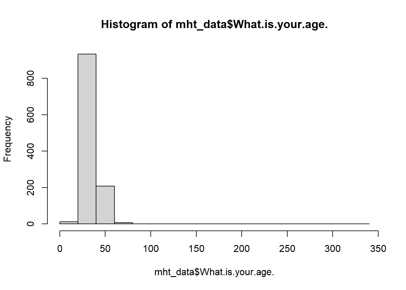 

The odd shae of this graph shows our outliers, it appears we may have a couple of low values and one very high value. We can further examine this using a boxplot.

#use the base r boxplot function to plot a boxplot of the age column
boxplot(mht_data$What.is.your.age.)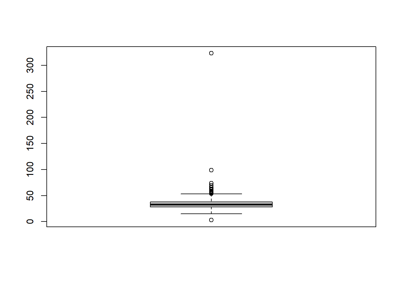 

The benefit of the boxplot if we can see the outliers (defined by the hollow circles) and we can identify we have 1 value greater than 300, 1 greater than 100 and one very small value. Personally, this is my preferred method to identify outliers.

Dealing with outliers

Now we understand where our outliers are siting we can look to handle them. One option, is to try and correct these values. In our case, this is not possible but if, for example, paper copies of the records were available these could be double checked and new values entered. However in our case, we are going to remove the values that are not plausible.

#remove values that are not plausible
#count how many rows are left
mht_data %>%
  filter(What.is.your.age. <100 & What.is.your.age. >= 18) %>%
  nrow()

## [1] 1157

We can see that by filtering our data to be less than 100 and older than 18 we lose 276 records. We may decide, based on an average retirement age of 70 we could further filter the data to include only records with this value.

#remove values that are not plausible
#count how many rows are left
mht_data %>%
  filter(What.is.your.age. <= 70 & What.is.your.age. >= 18) %>%
  nrow()

## [1] 1155

We can see that this only removes an additional 2 records making this choice likely best for this particular dataset.

It is always difficult to decide whether a value is low/high, or an outlier. In our case, we can justify our decision based on biology (people do not work past 100 very often if at all) and then retirement age (it is unlikely anyone works past 70). However, when such justification is not possible a rule of thumb that is often used is ±3 standard deviations. This value is not set in stone and other values can, and have, been used previously.