Magrittr

The magrittr package (named after the Belgium surrealist painter René Magritte) provides us the pipe function. The pipe function allows us to “pipe” a value forward into the next expression in our code. Lets take a look at some basic use cases so this idea can become more concrete.

One of the first things you may look to do after you have read a dataset into R is run the head function on it to examine the first few rows of data. This can be done as below.

For more information on the NHSRdatasets package, please check back to the creating variables post.

library(NHSRdatasets)
#the LOS_model is part of the NHSRdatasets package
#run the head function on it to examine the first few rows of data
head(LOS_model) 

##   ID Organisation Age LOS Death
## 1  1       Trust1  55   2     0
## 2  2       Trust2  27   1     0
## 3  3       Trust3  93  12     0
## 4  4       Trust4  45   3     1
## 5  5       Trust5  70  11     0
## 6  6       Trust6  60   7     0

We can see this generates the output we would expect. However, the same output can be achieved using the pipe or the ‘%>%’ set of symbols.

library(magrittr)
#the same action can be completed by using the pipe '%>%'
LOS_model %>%
  head()

##   ID Organisation Age LOS Death
## 1  1       Trust1  55   2     0
## 2  2       Trust2  27   1     0
## 3  3       Trust3  93  12     0
## 4  4       Trust4  45   3     1
## 5  5       Trust5  70  11     0
## 6  6       Trust6  60   7     0

We can see the pipe operators “pipes” the dataset into the head function. Personally, I often find it helpful to read the pipe symbol as “and then” when reading code. In the example above, this could read as: take the LOS_model dataset, and then execute the head function

Use case in data analysis

My favourite use of the pipe, and the one I use most often in my code, is to create a pipeline for data analysis using the pipe operator. In the example below, I use base R functions to generate a new variable, subset the dataset based on this variable before summarising the remaining data by generating a mean and standard deviation.

hospital_data <- LOS_model
hospital_data$log_age <- log(hospital_data$Age)
hospital_data <- subset(hospital_data, log_age > 4)
#we use <- to assign the LOS_model to the dataframe hospital_data
#we use the built in R function log() to calculate the natural logarithm of the column
#we use the base R subset function to filter our dataframe based on the logged age column
#we then use the R functions mean and sd to calculate the mean and standard deviation of this column
mean(hospital_data$Age, na.rm = TRUE)

## [1] 75.47973

sd(hospital_data$Age, na.rm = TRUE)

## [1] 11.86458

We can see that this is not very efficient, or easy to read code. It does the job very nicely but we create a lot of intermediary variables. There is also significant repetition in as much as we keep repeating the full name of the dataset usually on both sides of the assignment operator. This code can be simplified using the pipe.

It is also worth noting that you can also call the pipe from the dplyr package. So if you already have that package loaded, there is no need for magrittr.

library(dplyr)
#to reduce repetition and to simplify the code, you can use the pipe
#here we use the dplyr function filter in place of the base R subset function
LOS_model %>%
  mutate(log_age = log(Age)) %>%
  filter(log_age > 4) %>%
  summarise(
    mean = mean(Age, na.rm = TRUE),
    sd = sd(Age, na.rm = TRUE)
  ) %>%
  round(digits = 2)

## # A tibble: 1 x 2
##    mean    sd
##   <dbl> <dbl>
## 1  75.5  11.9

Whilst we do use a number of dplyr functions, we can see how the complexity of the code has decreased significantly with much less repeated code (the dataset name is only stated once in the first line of code). We can also see that we produce no intermediary products that would clutter our environment. Finally, the readability of the code has improved as the first word in each line is the function that we are wanting to perform. This means reading straight down the code we see the dataset we are taking, then we mutate a variable, then we filter, then we summarise the remaining data by creating a mean and standard deviation before rounding that information. At a glance, we can understand what the data pipeline is hoping to achieve.

Pipe and ggplot2

I believe it is worth briefly discussing the pipe operator and ggplot2. It is possible to pipe a dataframe into the ggplot function. Personally, I use this syntax extensively to perform a data manipulation, such as a summary, and then visualise this summary. An example can be seen below.

library(ggplot2)
#it is possible to pipe a dataframe into the ggplot function to graph the results
#the group by function from dplyr groups the dataset by the given variable
LOS_model %>%
  group_by(Death) %>%
  summarise(
    age = mean(Age, na.rm = TRUE)
  ) %>%
  ggplot(aes(x = Death, y = age)) +
  geom_col() +
  scale_x_continuous(breaks = c(0,1))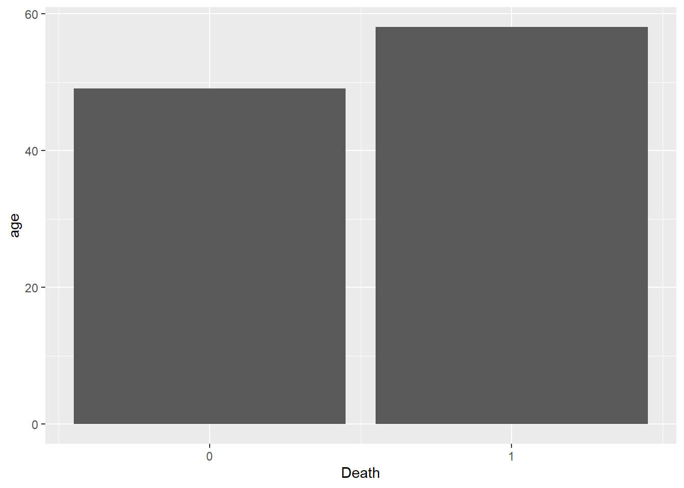

I take the LOS model, group the data by whether a participant is alive or dead, and then calculate the mean age of these two groups. I then pipe this data into ggplot and create a simple bar chart of the data. We can clearly see that participants who had died (1) were on average nearly 10 years older than their counterparts who survived.

It is worth noting, once you have used the pipe to get your data into the ggplot function, you will need to remember to shift back to using the + operator to add other ggplot2 functions such as geoms.

Hungry for more?

There are extensive more complex operations that the pipe operator can help simplify and some of these are outlined in the pipe documentation or R for Data Science.